Fitting a DAR model

This example creates an artificial signal with phase-amplitude coupling (PAC), fits a DAR model and show the modulation extracted in the DAR model.

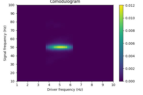
It also shows the comodulogram computed with a DAR model.

import numpy as np
import matplotlib.pyplot as plt

from pactools import Comodulogram
from pactools import simulate_pac
from pactools.dar_model import DAR, extract_driver

Let’s first create an artificial signal with PAC.

fs = 200.  # Hz
high_fq = 50.0  # Hz
low_fq = 5.0  # Hz
low_fq_width = 1.0  # Hz

n_points = 10000
noise_level = 0.4

signal = simulate_pac(n_points=n_points, fs=fs, high_fq=high_fq, low_fq=low_fq,
                      low_fq_width=low_fq_width, noise_level=noise_level,
                      random_state=0)

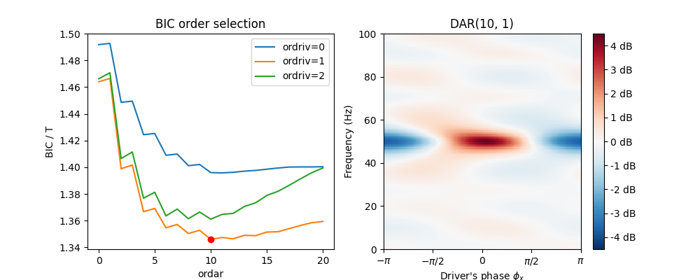
Extract a low-frequency band, and fit a DAR model, using BIC order selection.

# Prepare the plot for the two figures
fig, axs = plt.subplots(1, 2, figsize=(10, 4))
axs = axs.ravel()

# Extract a low frequency band
sigdriv, sigin, sigdriv_imag = extract_driver(
    sigs=signal, fs=fs, low_fq=low_fq, bandwidth=low_fq_width,
    extract_complex=True, random_state=0, fill=2)

# Create a DAR model
# Here we use BIC selection to get optimal hyperparameters (ordar, ordriv)
dar = DAR(ordar=20, ordriv=2, criterion='bic')
# Fit the DAR model
dar.fit(sigin=sigin, sigdriv=sigdriv, sigdriv_imag=sigdriv_imag, fs=fs)

# Plot the BIC selection
bic_array = dar.model_selection_criterions_['bic']
lines = axs[0].plot(bic_array)
axs[0].legend(lines, ['ordriv=%d' % d for d in [0, 1, 2]])
axs[0].set_xlabel('ordar')
axs[0].set_ylabel('BIC / T')
axs[0].set_title('BIC order selection')
axs[0].plot(dar.ordar_, bic_array[dar.ordar_, dar.ordriv_], 'ro')

# Plot the modulation extracted by the optimal model
dar.plot(ax=axs[1])
axs[1].set_title(dar.get_title(name=True))

Out:

Text(0.5, 1.0, 'DAR(10, 1)')

To compute a comodulogram, we perform the same steps for each low frequency: * Extract the low frequency * Fit a DAR model * Potentially with a model selection using the BIC * And quantify the PAC accross the spectrum.

Everything is handled by the class Comodulogram, by giving a (non-fitted) DAR model in the parameter method. Giving method='duprelatour' will default to DAR(ordar=10, ordriv=1, criterion=None), without BIC selection.

# Here we do not give the default set of parameter. Note that the BIC selection
# will be performed independantly for each model (i.e. at each low frequency).
dar = DAR(ordar=20, ordriv=2, criterion='bic')
low_fq_range = np.linspace(1, 10, 50)
estimator = Comodulogram(fs=fs, low_fq_range=low_fq_range,
                         low_fq_width=low_fq_width, method=dar,
                         progress_bar=False, random_state=0)
fig, ax = plt.subplots(1, 1, figsize=(6, 4))
estimator.fit(signal)
estimator.plot(axs=[ax])
ax.set_title('Comodulogram')

plt.show()

Out:

/home/tom/work/github/pactools/examples/plot_dar_model.py:86: UserWarning: Matplotlib is currently using agg, which is a non-GUI backend, so cannot show the figure.
  plt.show()