Surrogate analysis

This example shows how to estimate a significance threshold in a comodulogram.

A comodulogram shows the estimated PAC metric on a grid of frequency bands. In absence of PAC, a PAC metric will return values close to zero, but not exactly zero. To estimate if a value is significantly far from zero, we use a surrogate analysis.

In a surrogate analysis, we recompute the comodulogram many times, adding each time a random time shift to remove any possible coupling between the components. Nota that these time shifts have to be far from zero to effectively remove a potential coupling. These comodulograms give us an estimation of the fluctuation of the metric in the absence of PAC.

To derive a significance level from the list of comodulograms, we discuss here two different methods: - Computing a z-score on each couple of frequency, and thresholding at z = 4. - Computing a threshold at a given p-value, over a distribution of comodulogram maxima.

import numpy as np
import matplotlib.pyplot as plt

from pactools import Comodulogram
from pactools import simulate_pac

Let’s first create an artificial signal with PAC.

fs = 200.  # Hz
high_fq = 50.0  # Hz
low_fq = 5.0  # Hz
low_fq_width = 1.0  # Hz

n_points = 1000
noise_level = 0.4

signal = simulate_pac(n_points=n_points, fs=fs, high_fq=high_fq, low_fq=low_fq,
                      low_fq_width=low_fq_width, noise_level=noise_level,
                      random_state=0)

Then, let’s define the range of low frequency, and the PAC metric used.

low_fq_range = np.linspace(1, 10, 50)
method = 'duprelatour'  # or 'tort', 'ozkurt', 'penny', 'colgin', ...

We also choose the number of comodulograms computed in the surrogate analysis. A good rule of thumb is 10 / p_value. Example: 10 / 0.05 = 200.

n_surrogates = 200

As a surrogate analysis recquires to compute many comodulograms, the computation can be slow. If you have multiple cores in your CPU, you can leverage them using the parameter n_jobs > 1.

n_jobs = 1

To compute the comodulogram, we need to instanciate a Comodulogram object, then call the method fit. Adding the surrogate analysis is as simple as adding the n_surrogates parameter.

estimator = Comodulogram(fs=fs, low_fq_range=low_fq_range,
                         low_fq_width=low_fq_width, method=method,
                         n_surrogates=n_surrogates, progress_bar=True,
                         n_jobs=n_jobs)
estimator.fit(signal)

Out:

[                                        ] 0% | 0.00 sec | comodulogram: DAR(10, 1)
[                                        ] 2% | 2.92 sec | comodulogram: DAR(10, 1)
[.                                       ] 4% | 5.85 sec | comodulogram: DAR(10, 1)
[..                                      ] 6% | 8.78 sec | comodulogram: DAR(10, 1)
[...                                     ] 8% | 11.76 sec | comodulogram: DAR(10, 1)
[....                                    ] 10% | 14.80 sec | comodulogram: DAR(10, 1)
[....                                    ] 12% | 17.78 sec | comodulogram: DAR(10, 1)
[.....                                   ] 14% | 20.66 sec | comodulogram: DAR(10, 1)
[......                                  ] 16% | 23.62 sec | comodulogram: DAR(10, 1)
[.......                                 ] 18% | 26.81 sec | comodulogram: DAR(10, 1)
[........                                ] 20% | 30.32 sec | comodulogram: DAR(10, 1)
[........                                ] 22% | 35.13 sec | comodulogram: DAR(10, 1)
[.........                               ] 24% | 40.81 sec | comodulogram: DAR(10, 1)
[..........                              ] 26% | 44.83 sec | comodulogram: DAR(10, 1)
[...........                             ] 28% | 48.69 sec | comodulogram: DAR(10, 1)
[............                            ] 30% | 51.91 sec | comodulogram: DAR(10, 1)
[............                            ] 32% | 55.63 sec | comodulogram: DAR(10, 1)
[.............                           ] 34% | 58.93 sec | comodulogram: DAR(10, 1)
[..............                          ] 36% | 62.19 sec | comodulogram: DAR(10, 1)
[...............                         ] 38% | 65.18 sec | comodulogram: DAR(10, 1)
[................                        ] 40% | 68.08 sec | comodulogram: DAR(10, 1)
[................                        ] 42% | 71.60 sec | comodulogram: DAR(10, 1)
[.................                       ] 44% | 75.72 sec | comodulogram: DAR(10, 1)
[..................                      ] 46% | 79.59 sec | comodulogram: DAR(10, 1)
[...................                     ] 48% | 82.82 sec | comodulogram: DAR(10, 1)
[....................                    ] 50% | 86.43 sec | comodulogram: DAR(10, 1)
[....................                    ] 52% | 89.83 sec | comodulogram: DAR(10, 1)
[.....................                   ] 54% | 93.50 sec | comodulogram: DAR(10, 1)
[......................                  ] 56% | 97.07 sec | comodulogram: DAR(10, 1)
[.......................                 ] 58% | 100.72 sec | comodulogram: DAR(10, 1)
[........................                ] 60% | 103.99 sec | comodulogram: DAR(10, 1)
[........................                ] 62% | 107.60 sec | comodulogram: DAR(10, 1)
[.........................               ] 64% | 110.97 sec | comodulogram: DAR(10, 1)
[..........................              ] 66% | 114.53 sec | comodulogram: DAR(10, 1)
[...........................             ] 68% | 118.17 sec | comodulogram: DAR(10, 1)
[............................            ] 70% | 121.28 sec | comodulogram: DAR(10, 1)
[............................            ] 72% | 125.06 sec | comodulogram: DAR(10, 1)
[.............................           ] 74% | 128.19 sec | comodulogram: DAR(10, 1)
[..............................          ] 76% | 131.29 sec | comodulogram: DAR(10, 1)
[...............................         ] 78% | 134.33 sec | comodulogram: DAR(10, 1)
[................................        ] 80% | 137.74 sec | comodulogram: DAR(10, 1)
[................................        ] 82% | 141.35 sec | comodulogram: DAR(10, 1)
[.................................       ] 84% | 144.52 sec | comodulogram: DAR(10, 1)
[..................................      ] 86% | 147.83 sec | comodulogram: DAR(10, 1)
[...................................     ] 88% | 151.08 sec | comodulogram: DAR(10, 1)
[....................................    ] 90% | 154.34 sec | comodulogram: DAR(10, 1)
[....................................    ] 92% | 157.52 sec | comodulogram: DAR(10, 1)
[.....................................   ] 94% | 160.84 sec | comodulogram: DAR(10, 1)
[......................................  ] 96% | 164.17 sec | comodulogram: DAR(10, 1)
[....................................... ] 98% | 167.66 sec | comodulogram: DAR(10, 1)
[........................................] 100% | 170.84 sec | comodulogram: DAR(10, 1)

[........................................] 100% | 170.84 sec | comodulogram: DAR(10, 1)
<pactools.comodulogram.Comodulogram object at 0x7fb6f97287c0>

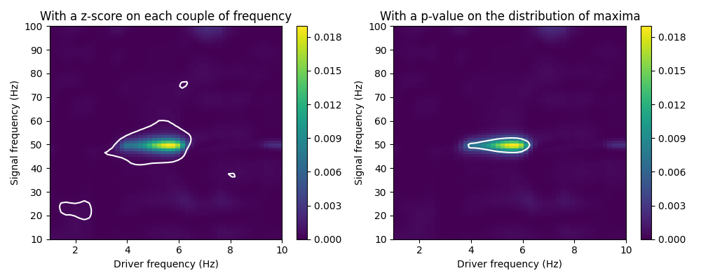
Then we plot the significance level on top of the comodulogram. Here we present two methods.

The z-score method presented here considers independently each pair of frequency of the comodulogram. For each pair, we compute the mean mu and standard deviation sigma of the PAC values computed over the surrogates signals. We then transform the original PAC values PAC (non time-shifted) into z-scores Z: Z = (PAC - mu) / sigma

This procedure, used for example in [Canolty et al, 2006], suffers from multiple-testing issues, and also assumes that the distribution of PAC values is Gaussian.

The other method presented here considers the ditribution of comodulogram maxima. For each surrogate comodulogram, we compute the maximum PAC value. From the obtained empirical distribution of maxima, we compute the 95-percentile, which corresponds to a p-value of 0.05.

This method does not assume the distribution to be Gaussian, nor suffers from multiple-testing issues. This is the default method in the plot method.

fig, axs = plt.subplots(1, 2, figsize=(10, 4))

z_score = 4.
estimator.plot(contour_method='z_score', contour_level=z_score,
               titles=['With a z-score on each couple of frequency'],
               axs=[axs[0]])

p_value = 0.05
estimator.plot(contour_method='comod_max', contour_level=p_value,
               titles=['With a p-value on the distribution of maxima'],
               axs=[axs[1]])

plt.show()

Out:

/home/tom/work/github/pactools/examples/plot_surrogate_analysis.py:109: UserWarning: Matplotlib is currently using agg, which is a non-GUI backend, so cannot show the figure.
  plt.show()

References

[Canolty et al, 2006] Canolty, R. T., Edwards, E., Dalal, S. S., Soltani, M., Nagarajan, S. S., Kirsch, H. E., … & Knight, R. T. (2006). High gamma power is phase-locked to theta oscillations in human neocortex. science, 313(5793), 1626-1628.