Peak-locking

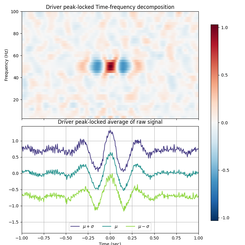
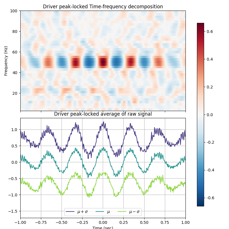
The peaks are extracted from the low frequency band, then both the raw-signal and a time-frequency representation are peak-locked and averaged.

Note the effect of the bandwidth low_fq_width on the number of oscillations in the results.

import matplotlib.pyplot as plt

from pactools import PeakLocking
from pactools import simulate_pac

Let’s first create an artificial signal with PAC.

fs = 200.  # Hz
high_fq = 50.0  # Hz
low_fq = 3.0  # Hz
low_fq_width = 2.0  # Hz

n_points = 10000
noise_level = 0.4
t_plot = 2.0  # sec

signal = simulate_pac(n_points=n_points, fs=fs, high_fq=high_fq, low_fq=low_fq,
                      low_fq_width=low_fq_width, noise_level=noise_level,
                      random_state=0)

Plot the amplitude of each frequency, locked with the peak of the slow wave

estimator = PeakLocking(fs=fs, low_fq=low_fq, low_fq_width=2.0, t_plot=t_plot)
estimator.fit(signal)
estimator.plot()

estimator = PeakLocking(fs=fs, low_fq=low_fq, low_fq_width=0.5, t_plot=t_plot)
estimator.fit(signal)
estimator.plot()

plt.show()

• 
• 

Out:

/home/tom/work/github/pactools/examples/plot_peak_locking.py:43: UserWarning: Matplotlib is currently using agg, which is a non-GUI backend, so cannot show the figure.
  plt.show()